Fixation indices
Introduction
Inbreeding
- “Consanguineous mating”
- Mating between relatives
- Positive assortative mating
- Extreme case: self-fertilization (e.g. Arabidopsis thaliana)

Self fertilization: heterozygosity
Self-fertilization & allele frequencies
- Recall:
- \(p = X + \frac{Y}{2}\)
- Generation 1
- \(X=0\), \(Y=1\)
- \(p = 0 + \frac{1}{2} = 0.5\)
- Generation 2
- \(X=0.25\), \(Y=0.5\)
- \(p = 0.25 + \frac{0.5}{2} = 0.5\)
Self-fertilization: summary
Fixation index
- Measures departure from Hardy-Weinberg frequencies
- Range -1 to +1
- +ve values, excess homozygotes
- -ve values, excess heterozygotes
- \(F = \frac{H_E - H_O}{H_E}\)
- \(H_E = 1 - \sum p_i^2\)
- \(H_O = \sum Y_i\)
Subdivided populations
Sources of departure from \(H_E\)
- Non-random mating within sub-populations (e.g. inbreeding)
- Wahlund effect: Allele frequency differences between sub‑populations
Fixation indices
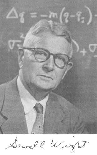
- Introduced by Sewall Wright
- Formulated for a dialleleic locus
- Hierarchical
- Can be applied to hierarchies of any depth
- Most common: 3 levels
- Total population
- Sub-populations
- Individuals in sub‑populations

Fixation indices
- \(F_{IS}\): Effect of non-random mating within subpopulations. Correlation of alleles in individuals, relative to sub-populations
- \(F_{ST}\): Magnitude of the Wahlund effect. Correlation of alleles within sub‑populations, relative to total population
- \(F_{IT}\): Combined effect of non-random mating and Wahlund effect. Correlation between alleles within individuals, relative to total population
Three measures of heterozygosity
\(H_I = \frac{\sum_{i=1}^n H_{O_i}}{n}\)
Average observed heterozygosity, frequency of heterozygous individuals
\(H_S = \frac{\sum_{i=1}^n 2p_iq_i}{n}\)
Average expected heterozygosity, among subpopulations
\(H_T = 2\bar{p}\bar{q}\)
\(H_T = 2 \left(\frac{\sum_{i=1}^n p_i}{n}\right) \left(\frac{\sum_{i=1}^n q_i}{n}\right)\)
Total expected heterozygosity
Defining fixation indices
- \(F_{IS} = \frac{H_S - H_I}{H_S}\)
- \(F_{ST} = \frac{H_T - H_S}{H_T}\)
- \(F_{IT} = \frac{H_T - H_I}{H_T}\)
\[1 - F_{IT} = \left(1-F_{ST}\right)\left(1-F_{IS}\right)\]
Numerical example
| \(p\) | \(2pq\) | \(H_O\) | |
|---|---|---|---|
| Population 1 | 0.3 | 0.42 | 0.418 |
| Population 2 | 0.5 | 0.50 | 0.480 |
| Population 3 | 0.8 | 0.32 | 0.336 |
Numerical example: \(H_I\)
| \(p\) | \(2pq\) | \(H_O\) | |
|---|---|---|---|
| Population 1 | 0.3 | 0.42 | 0.418 |
| Population 2 | 0.5 | 0.50 | 0.480 |
| Population 3 | 0.8 | 0.32 | 0.336 |
\[H_I = \frac{0.418 + 0.480 + 0.336}{3} = 0.4113\]
Numerical example: \(H_S\)
| \(p\) | \(2pq\) | \(H_O\) | |
|---|---|---|---|
| Population 1 | 0.3 | 0.42 | 0.418 |
| Population 2 | 0.5 | 0.50 | 0.480 |
| Population 3 | 0.8 | 0.32 | 0.336 |
\[H_S = \frac{0.42 + 0.50 + 0.32}{3} = 0.4133\]
Numerical example: \(H_T\)
| \(p\) | \(2pq\) | \(H_O\) | |
|---|---|---|---|
| Population 1 | 0.3 | 0.42 | 0.418 |
| Population 2 | 0.5 | 0.50 | 0.480 |
| Population 3 | 0.8 | 0.32 | 0.336 |
\[\bar{p} = \frac{0.3 + 0.5 + 0.8}{3} = 0.5333\]
\[\bar{q} = 1 - \bar{p} = 0.4667\]
\[H_T = 2 \times 0.5333 \times 0.4667 = 0.4978\]
Numerical example: Fixation indices
\[F_{IS} = \frac{0.4133 - 0.4113}{0.4133} = 0.0048\]
\[F_{ST} = \frac{0.4978 - 0.4133}{0.4978} = 0.1697\]
\[F_{IT} = \frac{0.4978 - 0.4113}{0.4978} = 0.1738\]
\(F_{ST}\)
- The most commonly-computed measure in population genetics
- Thousands of papers
- Measure of population subdivision / genetic divergence
- Range:
- 0 = Identical allele frequencies in all sub-populations
- 1 = Sub-populations fixed for different alleles
Estimating \(F_{ST}\)
- Need estimators of \(F_{ST}\)
- Sample data
- Multiple alleles, multiple loci
- Gene diversity
- Estimators of \(H\)
- \(G_{ST}\): Nei & colleagues
- Analysis of variance
- \(\theta\): Cockerham, Weir
- \(\phi_{ST}\): Excoffier & colleagues
\(F_{ST}\) and the coalescent
\[ F_{ST}=\frac{\bar{t}-\bar{t_0}}{\bar{t}}\]
- \(\bar{t}\): Average coalescence time for a pair of genes in the total sample
- For finite island model: \(\bar{t}=\left(\frac{1}{d}\bar{t_0}\right) + \left(\frac{d-1}{d}\bar{t_1}\right)\)
- \(\bar{t_0}\): Average coalescence time for a pair of genes sampled from the same deme
- \(\bar{t_1}\): Average coalescence time for a pair of genes sampled from different demes
- \(d\): number of demes (subpopulations)
Reading
Textbook: Pages 28 - 32; 118 - 130